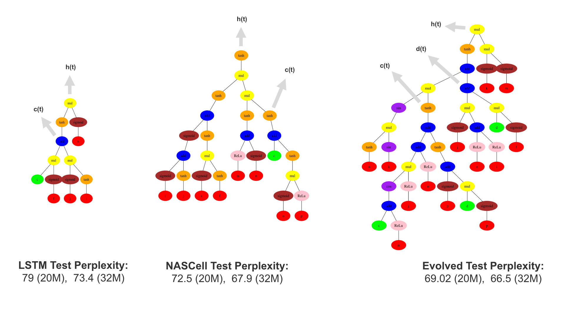
The Long Short-Term Memory (LSTM) model was originally developed in the early 1990s. Although it recently has turned out to be very useful in language tasks and sequence processing in general, it has changed very little over the last 25 years or so (Greff et al. 2017). Only recently, automated architecture search methods have started to discover that more complex variations could be more powerful.
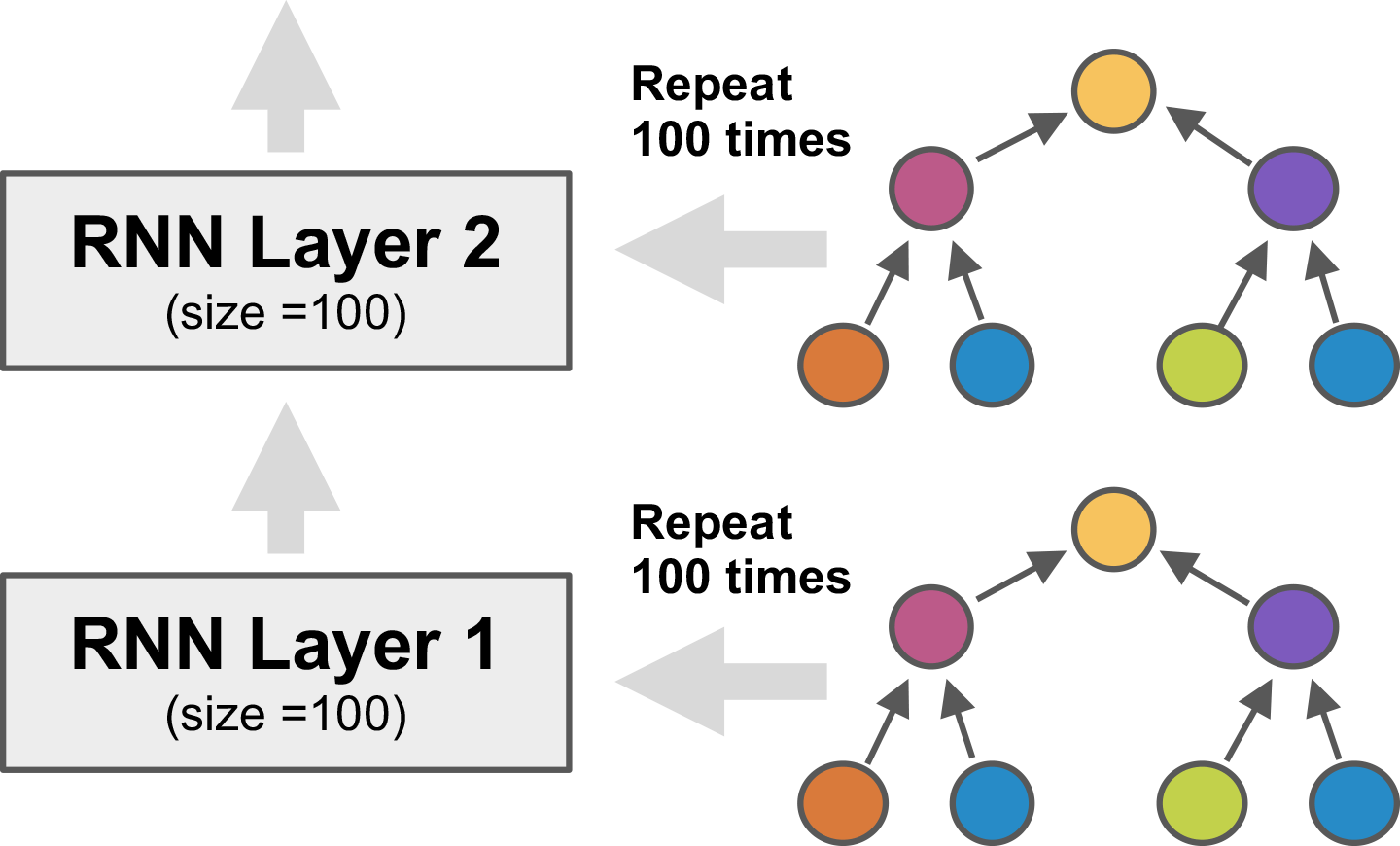
Neuroevolution is a particularly powerful such method, building on the exploratory power of evolutionary search. In particular, Paper 3 demonstrates that when the LSTM node architecture is represented as a tree, genetic programming (GP) methods can be used to evolve it effectively. It is also possible to encourage novelty by using an archive of already explored areas. Third, evaluation times can be reduced by training another LSTM network to predict the final validation performance from partial training. Only the structure of the LSTM node is evolved. The nodes are put together into a layered network, such as the one with two layers with 100 nodes each above that is then trained by gradient descent. In the experiments, such a network improved the state-of-the-art significantly in the standard language modeling benchmark, i.e. predicting the next word in a large text corpus. E.g. with 20M-parameter networks, it exceeded the performance of standard LSTM node by 10.8 perplexity points, and the performance of reinforcement-learning-based neural architecture search by 2.8 points.
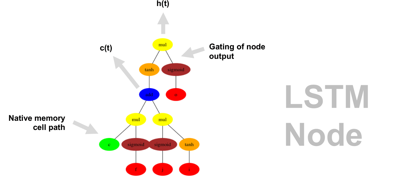
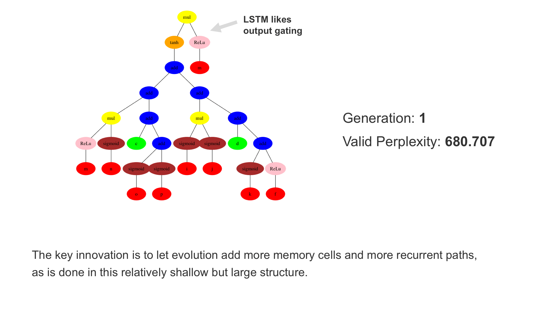
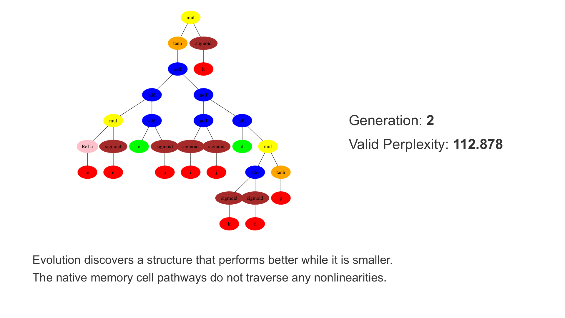
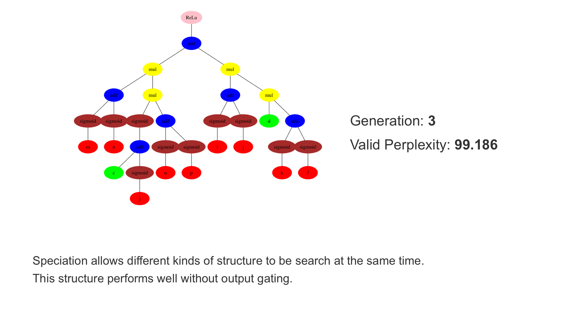
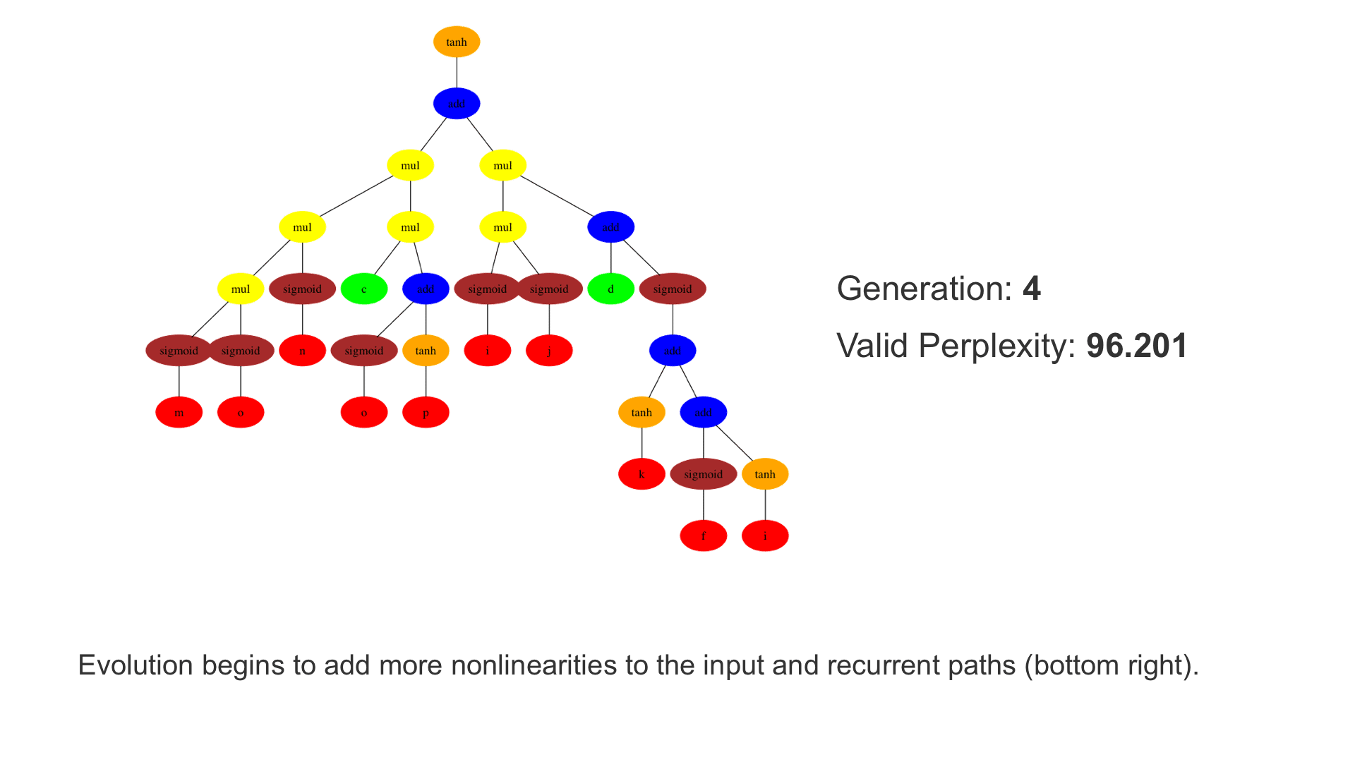
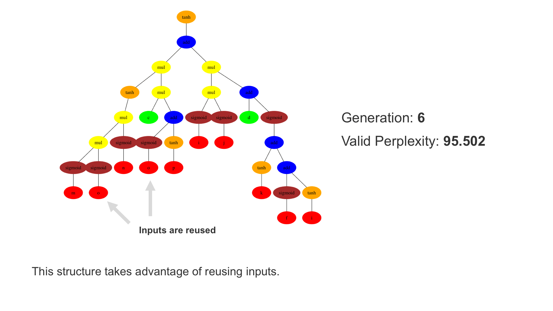
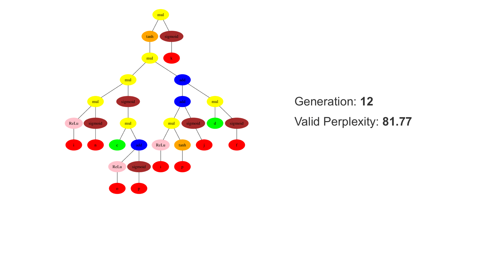
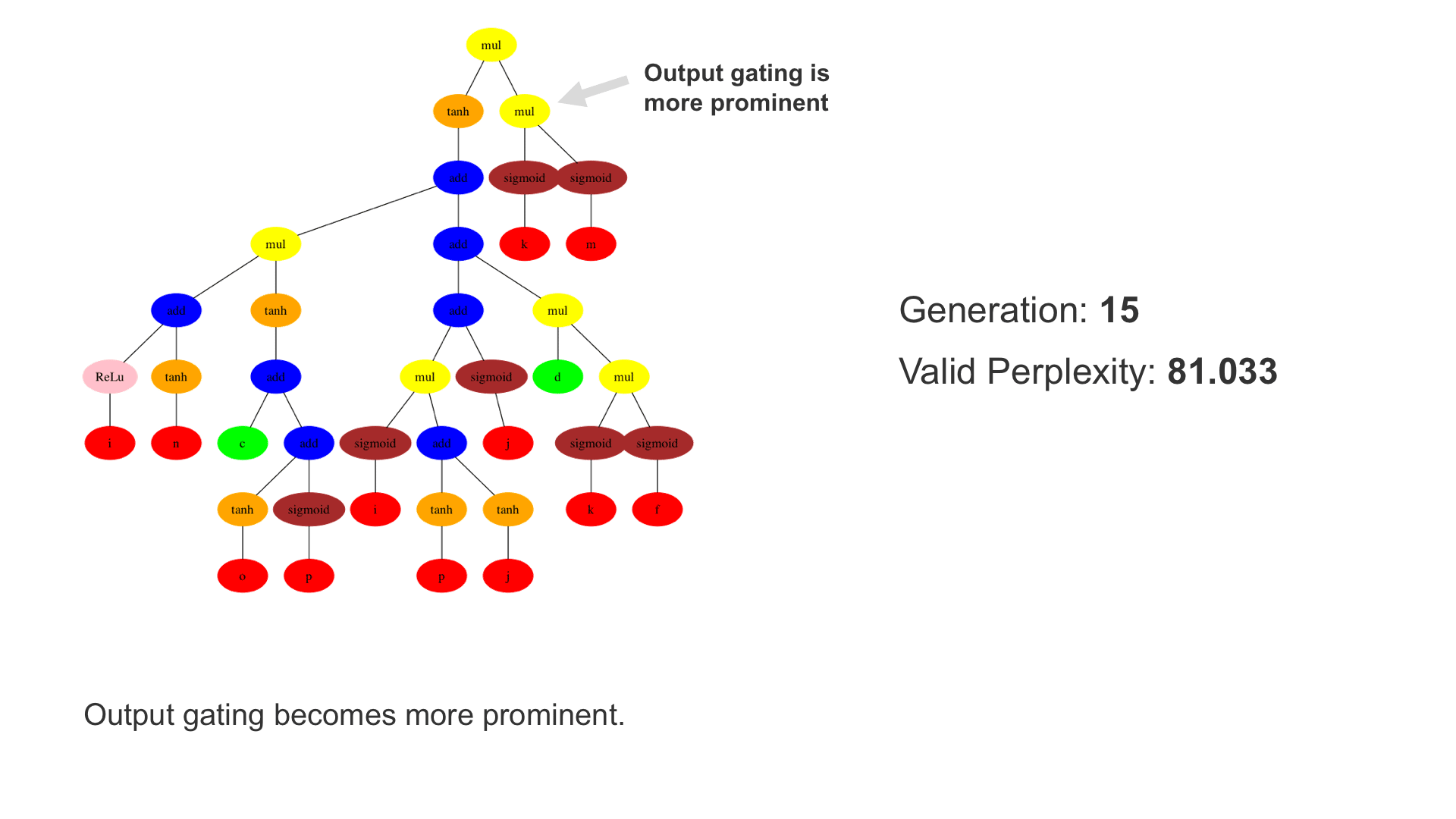
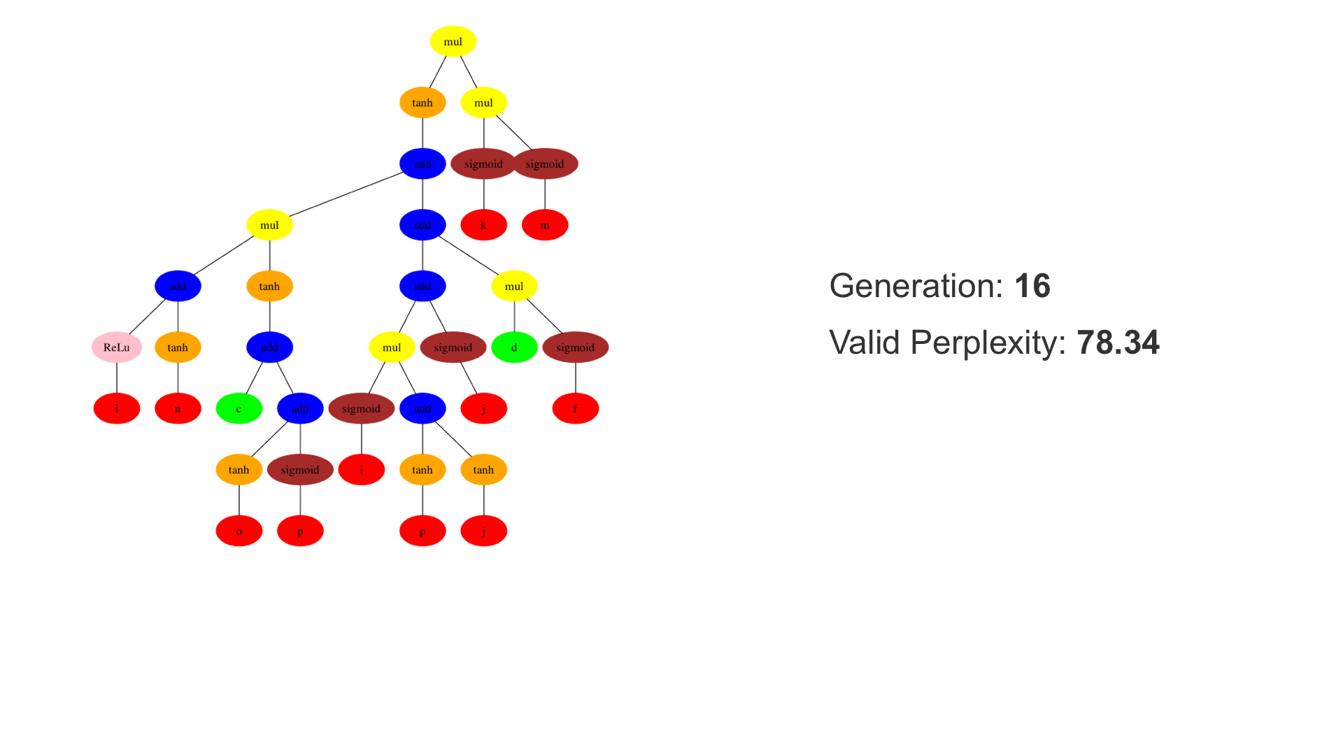
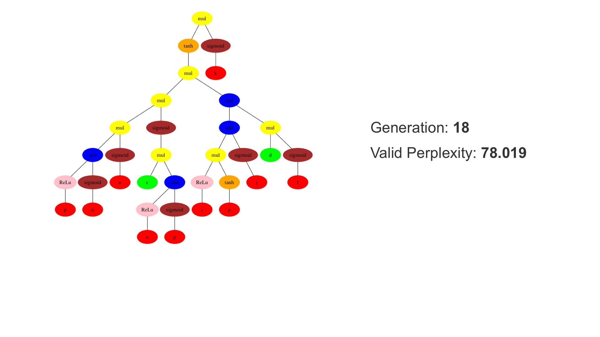
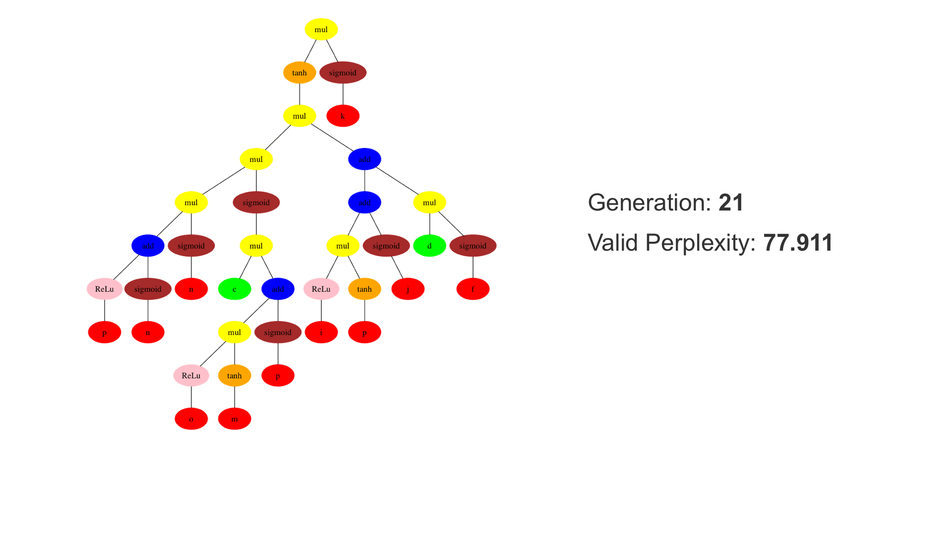
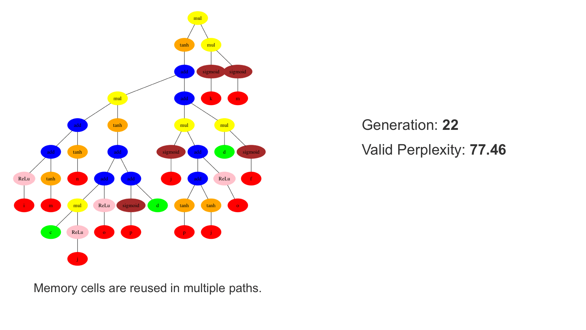
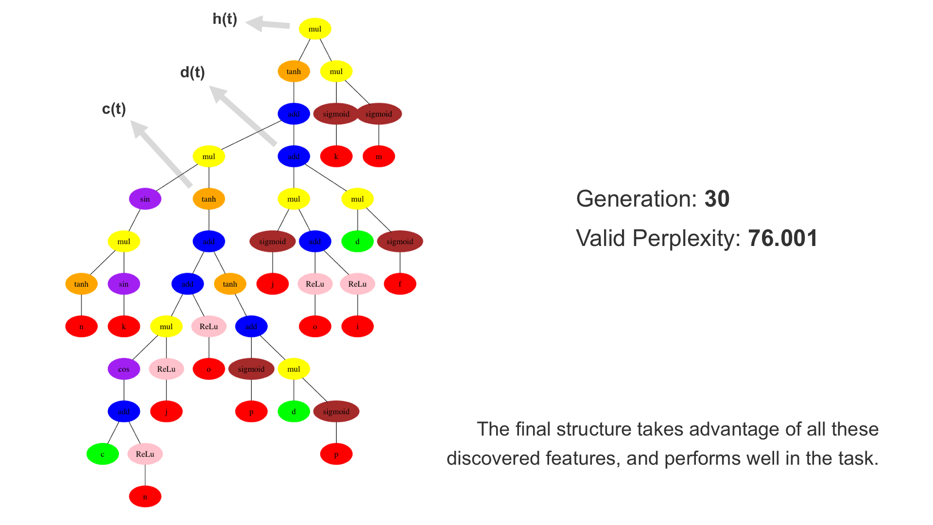
This demo shows how GP discovers an LSTM structure that achieves these results. The evolved tree structures are illustrated as shown above. This image depicts the structure of the standard LSTM as a tree five layers deep. The inputs are indicated by red circles, nonlinear transformations (sigmoid, tanh, ReLu) by brown, orange and pink, sum by blue, and multiplication by yellow. Multiplication establishes gating that controls the input, output, and recurrent paths. The native memory cell is shown by green; its output traverses only linear steps before the next output c(t), and is fed back to the memory cell in the next time step. This design means that its value is preserved and not squashed by nonlinearities. The internal connections have a weight of 1.0 and are not modified by gradient descent. The h(t) is the output of the node. Step through the animation below how evolution gradually complexifies the design and improves the performance!
